Introduction to the Marine Predators Algorithm

Overview

The Marine Predators Algorithm (MPA) is a nature-inspired metaheuristic optimization algorithm based on the foraging behavior of marine predators and their interactions with prey. It was introduced by Faramarzi et al. (2020) and has shown excellent performance on various optimization benchmarks.

Biological Inspiration

Marine predators use different movement strategies depending on the prey distribution:

Brownian motion: Short, random movements used when prey is abundant
Levy flight: Occasional long jumps followed by short movements, used when prey is scarce

The algorithm models these behaviors along with:

Memory: Predators remember successful foraging locations
FADs effect: Fish Aggregating Devices that can attract prey and predators

Algorithm Phases

MPA operates in three distinct phases based on the iteration count:

Phase 1: High Velocity Ratio (iterations 0 to Max_iter/3)

In this phase, the prey moves faster than the predator. The algorithm emphasizes exploration using Brownian motion. This helps discover promising regions in the search space.

Prey(t+1) = Prey(t) + P * R * stepsize

where stepsize = RB * (Elite - RB * Prey) and RB is Brownian random movement.

Phase 2: Unit Velocity Ratio (iterations Max_iter/3 to 2*Max_iter/3)

Predator and prey move at similar speeds. The population is split:

First half: Uses Brownian motion (exploitation around the elite)
Second half: Uses Levy flight (exploration)

This phase balances exploration and exploitation.

Phase 3: Low Velocity Ratio (iterations 2*Max_iter/3 to Max_iter)

The predator moves faster than the prey. All agents use Levy flight focused around the best solution, emphasizing exploitation to refine the solution.

Prey(t+1) = Elite + P * CF * stepsize

where stepsize = RL * (RL * Elite - Prey) and RL is Levy random movement.

Basic Usage

Installation

# From GitHub
remotes::install_github("urbs-dev/marinepredator")

Simple Optimization

library(marinepredator)

# Minimize the Sphere function (F01)
result <- mpa(
  SearchAgents_no = 30,   # Number of search agents
  Max_iter = 100,         # Maximum iterations
  lb = -100,              # Lower bound
  ub = 100,               # Upper bound
  dim = 10,               # Number of dimensions
  fobj = F01              # Objective function
)

print(result)
#> Marine Predators Algorithm Results:
#> -----------------------------------
#> Best fitness: 0.0008735510
#> Best position: 0.008820572 0.0083485218 0.008861006 -0.0111250684 0.0030944193 -0.0125384141 0.0115266286 0.0005965453 -0.0055542823 0.013889195
#> Convergence curve length: 100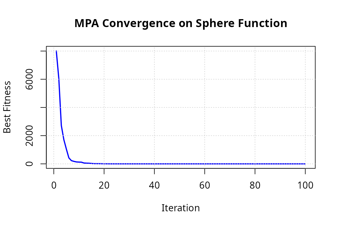

Visualizing Convergence

# Plot the convergence curve
plot(result$Convergence_curve, type = "l", col = "blue", lwd = 2,
     xlab = "Iteration", ylab = "Best Fitness",
     main = "MPA Convergence on Sphere Function")
grid()

Using Benchmark Functions

The package includes 23 standard benchmark functions:

# Get function details programmatically
details <- get_function_details("F09")  # Rastrigin function

# View the details
str(details)
#> List of 4
#>  $ lb  : num -5.12
#>  $ ub  : num 5.12
#>  $ dim : num 50
#>  $ fobj:function (x)

# Optimize the Rastrigin function
result_rastrigin <- mpa(
  SearchAgents_no = 30,
  Max_iter = 200,
  lb = details$lb,
  ub = details$ub,
  dim = 10,
  fobj = details$fobj
)

print(result_rastrigin)
#> Marine Predators Algorithm Results:
#> -----------------------------------
#> Best fitness: 4.7197635761
#> Best position: 0.0010936889 -0.0283214176 -0.9930850894 0.9814234412 -0.0412694518 0.0003992831 -0.0256177989 -0.0198230899 -0.9942359601 0.9943312343
#> Convergence curve length: 200

Custom Objective Functions

You can use MPA with any objective function:

# Define a custom function
# Minimum at (1, 2, 3)
custom_fun <- function(x) {
  sum((x - c(1, 2, 3))^2)
}

result_custom <- mpa(
  SearchAgents_no = 20,
  Max_iter = 100,
  lb = c(-10, -10, -10),
  ub = c(10, 10, 10),
  dim = 3,
  fobj = custom_fun
)

cat("Best position found:", round(result_custom$Top_predator_pos, 4), "\n")
#> Best position found: 1 2 3
cat("Best fitness:", result_custom$Top_predator_fit, "\n")
#> Best fitness: 1.383109e-10

Maximization Problems

MPA is a minimization algorithm. To maximize a function, negate its output:

# Function to maximize: f(x) = -sum(x^2)
# Maximum is at (0, 0, ..., 0) with value 0

result_max <- mpa(
  SearchAgents_no = 20,
  Max_iter = 100,
  lb = -10, ub = 10,
  dim = 5,
  fobj = function(x) sum(x^2)  # Minimize sum(x^2) = maximize -sum(x^2)
)

cat("Best position:", round(result_max$Top_predator_pos, 6), "\n")
#> Best position: 0.000179 -4e-05 -0.000218 8.8e-05 -7.9e-05
cat("Maximum value:", -result_max$Top_predator_fit, "\n")
#> Maximum value: -9.527871e-08

Algorithm Parameters

Key Parameters

Parameter	Description	Typical Values
`SearchAgents_no`	Number of search agents	20-50
`Max_iter`	Maximum iterations	100-500
`dim`	Problem dimensionality	Problem-dependent
`lb`, `ub`	Search space bounds	Problem-dependent

Internal Parameters (not exposed)

FADs = 0.2: Fish Aggregating Devices effect probability
P = 0.5: Movement probability controlling step size

Guidelines for Parameter Selection

SearchAgents_no: Use more agents for complex, multimodal problems
Max_iter: Increase for high-dimensional problems
Bounds: Set tight bounds if domain knowledge is available

Comparing Functions

# Compare MPA performance on different functions
set.seed(42)  # For reproducibility

functions <- c("F01", "F05", "F09", "F10")
results <- list()

for (func_name in functions) {
  details <- get_function_details(func_name)
  result <- mpa(
    SearchAgents_no = 30,
    Max_iter = 100,
    lb = details$lb,
    ub = details$ub,
    dim = min(details$dim, 20),  # Limit dimensions for speed
    fobj = details$fobj
  )
  results[[func_name]] <- result$Top_predator_fit
}

# Display results
data.frame(
  Function = names(results),
  Best_Fitness = unlist(results)
)
#>     Function Best_Fitness
#> F01      F01    0.1110520
#> F05      F05   22.1944567
#> F09      F09   21.6414587
#> F10      F10    0.2116683

Logging

You can enable logging to track optimization progress:

result <- mpa(
  SearchAgents_no = 30,
  Max_iter = 100,
  lb = -100, ub = 100,
  dim = 10,
  fobj = F01,
  logFile = "mpa_log.txt"
)

References

Faramarzi, A., Heidarinejad, M., Mirjalili, S., & Gandomi, A. H. (2020). Marine Predators Algorithm: A Nature-inspired Metaheuristic. Expert Systems with Applications, 152, 113377. https://doi.org/10.1016/j.eswa.2020.113377

Marc Grossouvre

2026-02-02